library(ThinkingGrid)
library(lme4)
#> Loading required package: Matrix
library(sjPlot)
library(png)
library(grid)

data_file <- system.file("extdata", "sample_data.csv", package = "ThinkingGrid")
tg_data <- read.csv(data_file)

knitr::kable(head(tg_data))| id | condition | probe | dc | ac | valence |
|---|---|---|---|---|---|
| 0 | Negative | 1 | 6 | 1 | -1 |
| 0 | Negative | 2 | 4 | 3 | -1 |
| 0 | Negative | 3 | 3 | 3 | 0 |
| 0 | Negative | 4 | 4 | 5 | 0 |
| 1 | Negative | 1 | 5 | 1 | -2 |
| 1 | Negative | 2 | 5 | 1 | -2 |
In case data is already collected, users can automatically add the
quadrant depths using the add_depths function. The
deliberate and automatic constraints column names must be passed to the
function and must range from one to six for it to work correctly.
tg_data <- add_depths(
  tg_data,
  dc = "dc",
  ac = "ac"
)

knitr::kable(head(tg_data))| id | condition | probe | dc | ac | valence | total_depth | quadrant | sticky | hybrid | free | directed |
|---|---|---|---|---|---|---|---|---|---|---|---|
| 0 | Negative | 1 | 6 | 1 | -1 | 5 | 3 | 0 | 0 | 0 | 5 |
| 0 | Negative | 2 | 4 | 3 | -1 | 1 | 3 | 0 | 0 | 0 | 1 |
| 0 | Negative | 3 | 3 | 3 | 0 | 1 | 1 | 0 | 0 | 1 | 0 |
| 0 | Negative | 4 | 4 | 5 | 0 | 2 | 4 | 0 | 2 | 0 | 0 |
| 1 | Negative | 1 | 5 | 1 | -2 | 4 | 3 | 0 | 0 | 0 | 4 |
| 1 | Negative | 2 | 5 | 1 | -2 | 4 | 3 | 0 | 0 | 0 | 4 |
The depths can be used as dependent variables in statistical
analyses. The thinkgrid_quadrant_plot function provides a
convenient way to visualize each of these analyses within their
individual quadrants. Build the models and their respective ggplot2
objects similar to the example shown below.
free_model <- lmer(free ~ valence + (1|id), data = tg_data)
sticky_model <- lmer(sticky ~ valence + (1|id), data = tg_data)
directed_model <- lmer(directed ~ valence + (1|id), data = tg_data)
salience_model <- lmer(hybrid ~ valence + (1|id), data = tg_data)

free_plot <- plot_model(free_model, type = "pred")
sticky_plot <- plot_model(sticky_model, type = "pred")
directed_plot <- plot_model(directed_model, type = "pred")
salience_plot <- plot_model(salience_model, type = "pred")
Once the plots are made, simply pass them to the
thinkgrid_quadrant_plot function.
combined_plot1 <- thinkgrid_quadrant_plot(
  p_sticky = sticky_plot,
  p_salience = salience_plot,
  p_free = free_plot,
  p_directed = directed_plot
)

combined_plot1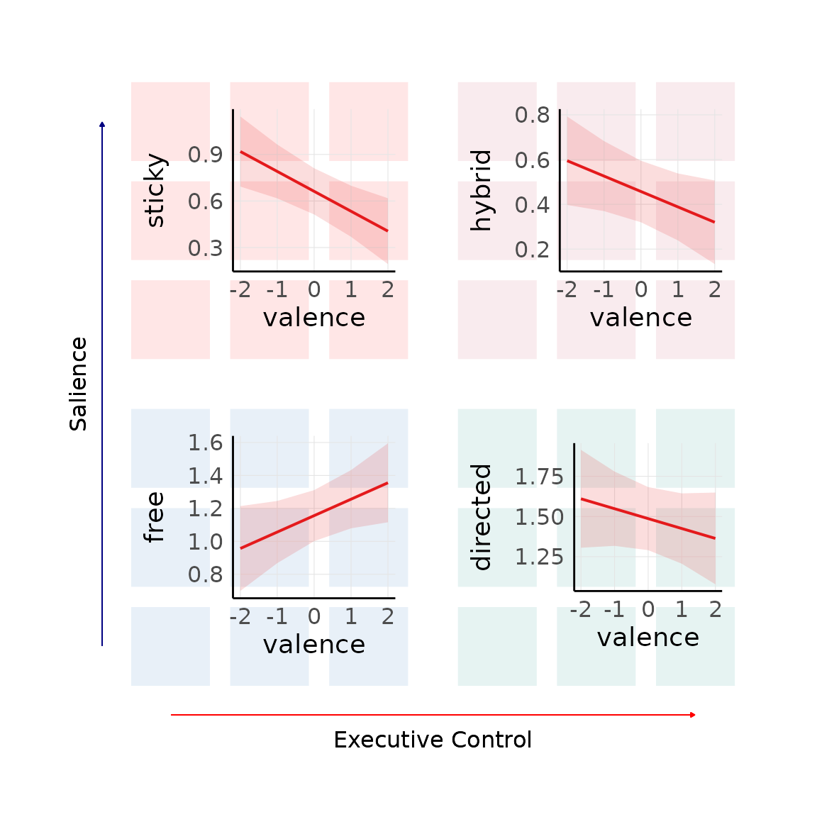
This function also accepts images as arguments, as long as they are transparent (e.g., png). Instead of passing the ggplot2 objects, the png object can be passed instead.
image_file <- system.file("extdata", "rabbiduck.png", package = "ThinkingGrid")
image <- readPNG(image_file)
image <- rasterGrob(image)

combined_plot2 <- thinkgrid_quadrant_plot(
  p_sticky = image,
  p_salience = salience_plot,
  p_free = image,
  p_directed = directed_plot
)

combined_plot2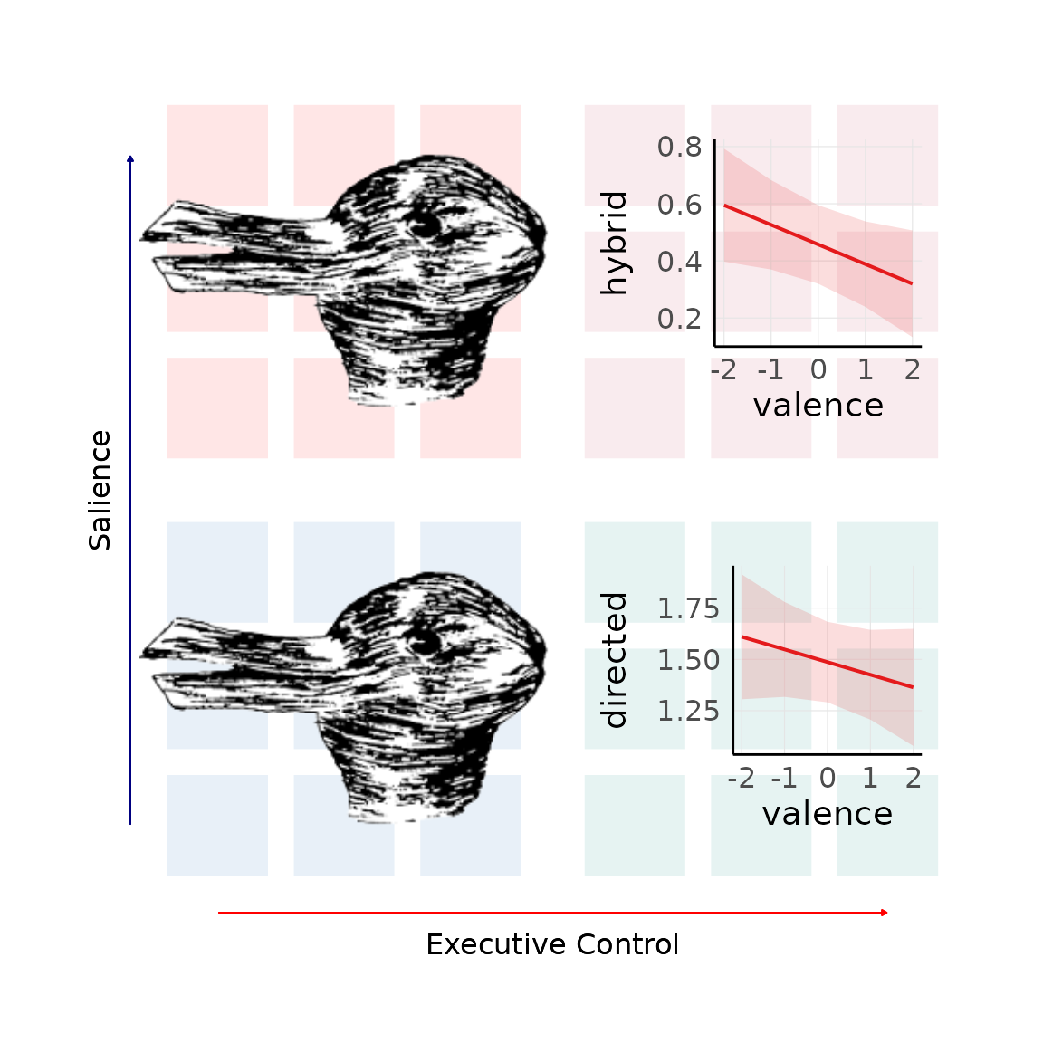
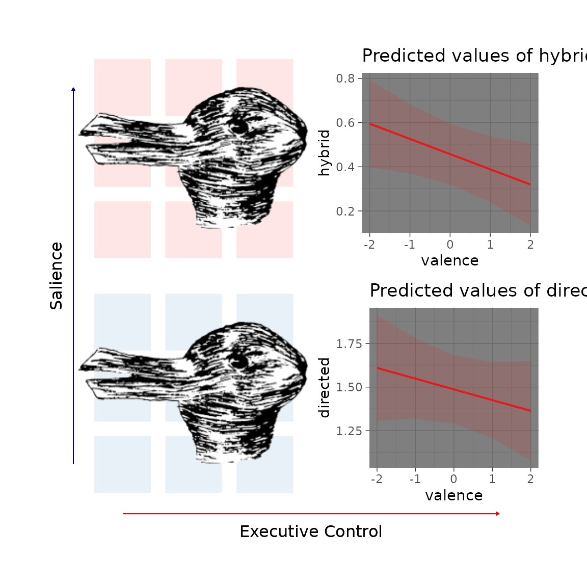
Plotting Quirks
You will notice that the theme of the argument plots is different than the theme of the subplots. This is because, by default, the inner theme (i.e., subplot theme) is generated by
default_inner_theme
#> function (inner_margin = 20)
#> {
#>     im <- inner_margin
#>     ggplot2::theme_minimal() + ggplot2::theme(plot.background = ggplot2::element_blank(),
#>         panel.background = ggplot2::element_blank(), plot.margin = ggplot2::margin(im,
#>             im, im, im), legend.position = "none", aspect.ratio = 1,
#>         axis.title = ggplot2::element_text(size = 14), axis.text = ggplot2::element_text(size = 12),
#>         axis.title.y = ggplot2::element_text(margin = ggplot2::margin(r = 10)),
#>         panel.grid.major = ggplot2::element_line(color = "gray90",
#>             linewidth = 0.2), panel.grid.minor = ggplot2::element_blank(),
#>         axis.line = ggplot2::element_line(color = "black", linewidth = 0.5)) +
#>         ggplot2::labs(title = ggplot2::element_blank())
#> }
#> <bytecode: 0x55b3cbe3c028>
#> <environment: namespace:ThinkingGrid>
You can manually set the inner theme using the
inner_theme optional argument. This will not affect png
images, only the plots.
library(ggplot2)
#>
#> Attaching package: 'ggplot2'
#> The following object is masked from 'package:sjPlot':
#>
#>     set_theme

thinkgrid_quadrant_plot(
  p_sticky = image,
  p_salience = salience_plot,
  p_free = image,
  p_directed = directed_plot,
  inner_theme = ggplot2::theme_dark()
)
Rendering
If you are using RStudio, plots generated by
thinkgrid_quadrant_plot have a tendency to not render
especially nicely (funny aspect ratios, text crowding issues, etc). To
solve such rendering issues, we recommend saving the plot to a file.
ggplot2::ggsave("properly_rendered.jpg", combined_plot2, width = 10, height = 10, dpi = 300)